Getting started with Kinesis
In this notebook, we will generate a mock cluster, observe (add noise) and fit to see if we recover the true parameters of its internal kinematics.
Notes on dependences - gapipes: for custom pandas accessor g to get covariance matrices, astropy coordinate objects.. - arviz: for visualization
[1]:
%matplotlib inline
import matplotlib.pyplot as plt
from matplotlib import colors
import pandas as pd
import numpy as np
import astropy.units as u
import astropy.coordinates as coords
import arviz as az

# project dependencies
import gapipes as gp
import kinesis as kn
[2]:
np.random.seed(18324)
Making and observing a mock cluster
First, let’s make a cluster with some fiducial parameters.
[4]:
N = 150  # number of sources
b0 = np.array([17.7, 41.2, 13.3])    # pc
v0 = np.array([-6.32, 45.24, 5.30])  # [vx, vy, vz] in km/s
sigv = 1.  # dispersion, km/s

cl = kn.Cluster(v0, sigv, b0=b0)
The cluster currently has no members. We need to ‘sample’ the cluster in order to populate it. There are two methods for sampling a cluster: - sample_sphere: sampling uniformly within a maximum radius - sample_at: sample at exactly the positions you want by giving it astropy coordinates.
Let’s do uniform sphere for now. All normal methods of Cluster will return itself with modified attributes for method chaining. Sampling will modify its members from None to an instance of ClusterMembers.
[6]:
cl.sample_sphere(N=N, Rmax=5)
cl.members
[6]:
<kinesis.mock.ClusterMembers at 0x7ff1b8b9bc50>
There are two Gaia-like DataFrame associated with ClusterMembers: - truths: this is the noise-free Gaia data consistent with the Cluster’s internal motions - observed: this is the noise-added Gaia data. If the ClusterMembers has not been observed, it will be None.
Now let’s observe the cluster. In order to observe, you need to specify the 3x3 covariance matrix for (parallax, pmra, pmdec) with cov keyword. If cov is (3,3) array, this will be assumed for all stars. You can also specify different covariance matrix for different stars by specifying cov to be (N, 3, 3) array. The noise model is assumed to be Gaussian.
It is also possible to specify covariance by giving another Gaia-like data frame using error_from keyword. The following columns needed to construct to covariance matrix are expected: parallax_error, pmra_error, pmdec_error, parallax_pmra_corr, parallax_pmdec_corr, pmra_pmdec_corr. This is useful, for example, if you want to simulate data as noisy as the actual Gaia data you want to model.
Radial velocity errors should be specified separately with rv_error keyword, which should be 1-d array with N elements, each specifying the Gaussian standard deviation in km/s. If any element in rv_error is np.nan, it is assumed that the star does not have RV measurement.
This will add noise to the astrometry and radial velocities of the cluster members, and the noise-added Gaia-like data frame is now accessible with cl.members.observed.
Let’s specify simply 0.01 mas or mas/yr errors for parallax and pmra/pmdec and no available RVs.
[8]:
cl.observe(cov=np.eye(3)*0.01)
[8]:
Cluster(b0=[17.7 41.2 13.3], v0=[-6.32 45.24 5.3 ], sigmav=1.0)
[9]:
cl.members.observed.head()
[9]:
| ra | dec | parallax | pmra | pmdec | parallax_pmra_corr | parallax_pmdec_corr | pmra_pmdec_corr | parallax_error | pmra_error | pmdec_error | |
|---|---|---|---|---|---|---|---|---|---|---|---|
| 0 | 69.827908 | 15.519434 | 21.658627 | 100.052890 | -26.044631 | 0.0 | 0.0 | 0.0 | 0.1 | 0.1 | 0.1 |
| 1 | 63.449065 | 18.338080 | 20.766187 | 116.685278 | -26.140222 | 0.0 | 0.0 | 0.0 | 0.1 | 0.1 | 0.1 |
| 2 | 67.364160 | 20.868653 | 21.499381 | 97.637078 | -44.203983 | 0.0 | 0.0 | 0.0 | 0.1 | 0.1 | 0.1 |
| 3 | 62.220135 | 16.061914 | 20.091140 | 116.236887 | -26.155718 | 0.0 | 0.0 | 0.0 | 0.1 | 0.1 | 0.1 |
| 4 | 61.149763 | 17.653502 | 22.460105 | 124.989805 | -28.335939 | 0.0 | 0.0 | 0.0 | 0.1 | 0.1 | 0.1 |
Fitting the mock data
Now let’s try to fit the mock data that we generated. Under the hood, kinesis uses stan using its python interface pystan.
[8]:
fitter = kn.Fitter(include_T=False, recompile=True)
INFO:pystan:COMPILING THE C++ CODE FOR MODEL anon_model_47c60c044460f8a93fb3bb3ea5a6ba35 NOW.
INFO:kinesis.models:Compiling general_model
[9]:
df = cl.members.observed.copy()
fit = fitter.fit(df, sample=False)
print(f"v0, sigv = {fit['v0']}, {fit['sigv']:.4f}")
print(f"diff from truth: {fit['v0']-v0}, {fit['sigv']-sigv:.4f}")
v0, sigv = [-6.0485426  45.77930913  5.55432163], 0.9072
diff from truth: [0.2714574  0.53930913 0.25432163], -0.0928
[10]:
stanfit = fitter.fit(df)
[14]:
stanfit.azfit
[14]:
Inference data with groups:
        > posterior
        > sample_stats
        > observed_data
[15]:
azfit=stanfit.azfit
[19]:
az.summary(azfit, var_names=['v0','sigv'])
[19]:
| mean | sd | hpd_3% | hpd_97% | mcse_mean | mcse_sd | ess_mean | ess_sd | ess_bulk | ess_tail | r_hat | |
|---|---|---|---|---|---|---|---|---|---|---|---|
| v0[0] | -6.060 | 0.434 | -6.856 | -5.228 | 0.011 | 0.008 | 1615.0 | 1607.0 | 1625.0 | 2122.0 | 1.0 |
| v0[1] | 45.754 | 1.000 | 43.927 | 47.715 | 0.025 | 0.018 | 1632.0 | 1632.0 | 1640.0 | 2098.0 | 1.0 |
| v0[2] | 5.546 | 0.328 | 4.920 | 6.143 | 0.008 | 0.006 | 1649.0 | 1649.0 | 1653.0 | 1991.0 | 1.0 |
| sigv | 0.919 | 0.037 | 0.850 | 0.990 | 0.001 | 0.000 | 5188.0 | 5174.0 | 5183.0 | 3203.0 | 1.0 |
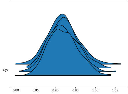
[16]:
az.plot_forest(azfit, kind='ridgeplot', var_names=['sigv']);
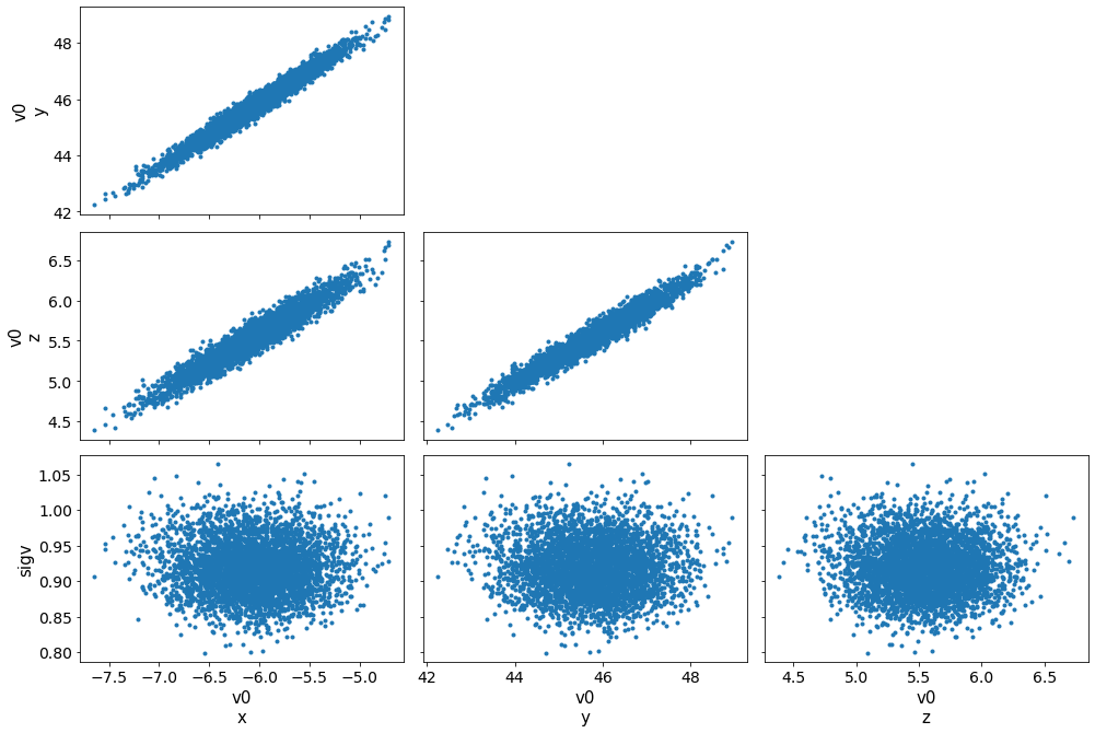
[21]:
az.plot_pair(azfit, var_names=['v0','sigv']);
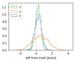
[12]:
v0_diff = stanfit['v0'] - cl.v0[None,:]

plt.figure(figsize=(4,3))
plt.hist(v0_diff, bins=64, histtype='step', density=True, label=['x','y','z']);
plt.xlabel("diff from truth [km/s]");
plt.legend(loc='upper left');
plt.axvline(0, c='gray', lw=.5);
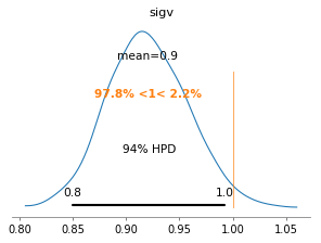
[13]:
az.plot_posterior(azfit, var_names=['sigv'], ref_val=cl.sigmav, figsize=(4,3));
[14]:
# plt.figure(figsize=(4,3))
# g = np.einsum('ni,nij,nj->n', a-r['a_model'], np.linalg.inv(C), a-r['a_model'])

# plt.hist(g, 32, density=True);
# plt.hist(g, np.logspace(0, 4, 32), density=True);
# plt.xscale('log');
# plt.yscale('log')
Basic cluster model with partial RVs
[15]:
N = 150
b0 = np.array([17.7, 41.2, 13.3])    # pc
v0 = np.array([-6.32, 45.24, 5.30])
sigv = 1.

cl = kn.Cluster(v0, sigv, b0=b0)\
       .sample_sphere(N=N, Rmax=5)\
       .observe(cov=np.eye(3)*0.01)

# Give random half of the stars RV with 0.5 km/s uncertainty
Nrv = int(N*0.5)
rv_error = 0.5
irand = np.random.choice(np.arange(N), size=Nrv, replace=False)

df = cl.members.observed.copy()
df['radial_velocity'] = np.random.normal(cl.members.truth['radial_velocity'].values, rv_error)
df['radial_velocity_error'] = rv_error
[16]:
df = cl.members.observed.copy()
fit = fitter.fit(df, sample=False)
print(f"v0, sigv = {fit['v0']}, {fit['sigv']:.4f}")
print(f"diff from truth: {fit['v0']-v0}, {fit['sigv']-sigv:.4f}")
v0, sigv = [-5.92897309 46.06913061  5.49316135], 0.9835
diff from truth: [0.39102691 0.82913061 0.19316135], -0.0165
[17]:
stanfit_partialrv = fitter.fit(df)
[18]:
# workaround for a bug in arviz instantiating InferenceData
d = stanfit_partialrv.extract(permuted=False, pars=['v0', 'sigv'])
d = {k:np.swapaxes(v, 0, 1) for k,v in d.items()}
azfit_partialrv = az.from_dict(d)
[19]:
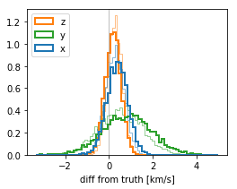
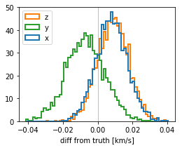
v0_diff0 = stanfit['v0'] - cl.v0[None,:]
v0_diff = stanfit_partialrv['v0'] - cl.v0[None,:]

plt.figure(figsize=(4,3))
color = ['tab:blue', 'tab:green', 'tab:orange']
plt.hist(v0_diff0, bins=64, histtype='step', density=True, color=color, lw=.5);
plt.hist(v0_diff, bins=64, histtype='step', density=True, color=color, label=['x','y','z'], lw=2);
plt.xlabel("diff from truth [km/s]");
plt.legend(loc='upper left');
plt.axvline(0, c='gray', lw=.5);
[20]:
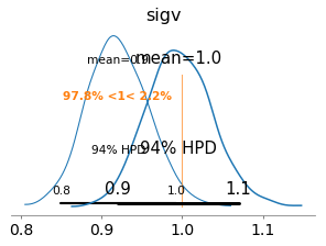
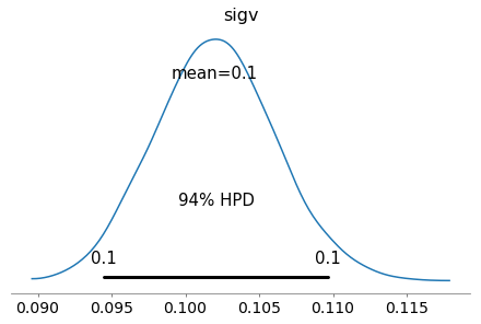
axs = az.plot_posterior(azfit, var_names=['sigv'], ref_val=cl.sigmav, figsize=(4,3))
az.plot_posterior(azfit_partialrv, var_names=['sigv'], ax=axs);
Cluster with rotation
[21]:
N = 150
b0 = np.array([17.7, 41.2, 13.3])    # pc
v0 = np.array([-6.32, 45.24, 5.30])
sigv = 1.
omegas = [40., 20., 50.]

cl = kn.Cluster(v0, sigv, b0=b0, omegas=omegas)\
       .sample_sphere(N=N, Rmax=15)\
       .observe(cov=np.eye(3)*0.001)
cl0 = kn.Cluster(v0, sigv, b0=b0).sample_at(cl.members.truth.g.icrs)

# Give random half of the stars RV with 0.5 km/s uncertainty
Nrv = int(N*0.5)
rv_error = 0.5
irand = np.random.choice(np.arange(N), size=Nrv, replace=False)

df = cl.members.observed.copy()
df['radial_velocity'] = np.random.normal(cl.members.truth['radial_velocity'].values, rv_error)
df['radial_velocity_error'] = rv_error
[22]:
m = kn.Fitter(include_T=True)
fit = m.fit(df, sample=False, b0=b0)
INFO:kinesis.models:Reading model from disk
[23]:
print(f"v0, sigv = {fit['v0']}, {fit['sigv']:.4f}")
print(f"diff from truth: {fit['v0']-v0}, {fit['sigv']-sigv:.4f}")
print(f"{fit['T_param']}")
print(f"{cl.T}")
v0, sigv = [-6.382561   45.25883593  5.52632739], 0.9632
diff from truth: [-0.062561    0.01883593  0.22632739], -0.0368
[[ -5.47942742 -48.81690422  14.15808424]
 [ 27.02856238   6.34378433 -29.12948134]
 [ -4.03730063  37.49138498  -3.81971577]]
[[  0. -50.  20.]
 [ 50.   0. -40.]
 [-20.  40.   0.]]
[ ]:
# omegax = 0.5*(r['T_param'][2, 1] - r['T_param'][1, 2])
# omegay = 0.5*(r['T_param'][0, 2] - r['T_param'][2, 0])
# omegaz = 0.5*(r['T_param'][1, 0] - r['T_param'][0, 1])

# w1 = 0.5*(r['T_param'][2, 1] + r['T_param'][1, 2])
# w2 = 0.5*(r['T_param'][0, 2] + r['T_param'][2, 0])
# w3 = 0.5*(r['T_param'][1, 0] + r['T_param'][0, 1])
# w4 = r['T_param'][0, 0]
# w5 = r['T_param'][1, 1]
# kappa = w4 + w5 + r['T_param'][2, 2]
# print(omegax, omegay, omegaz)
# print(w1, w2, w3)
# print(w4, w5)
# print(kappa)
[25]:
stanfit = m.fit(df, b0=b0)
[26]:
azfit = az.from_pystan(stanfit)
[27]:
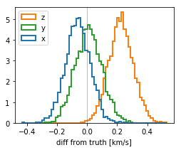
v0_diff = stanfit['v0'] - cl.v0[None,:]

plt.figure(figsize=(4,3))
color = ['tab:blue', 'tab:green', 'tab:orange']
plt.hist(v0_diff, bins=64, histtype='step', density=True, color=color, label=['x','y','z'], lw=2);
plt.xlabel("diff from truth [km/s]");
plt.legend(loc='upper left');
plt.axvline(0, c='gray', lw=.5);
[28]:
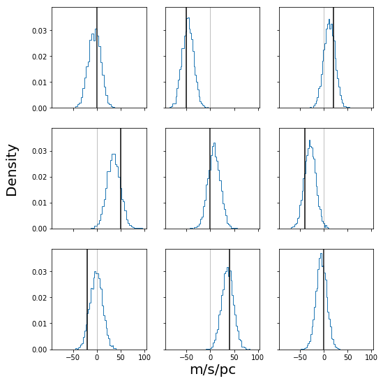
fig, ax = plt.subplots(3, 3, figsize=(8, 8), sharex=True, sharey=True)
fig.subplots_adjust(bottom=0.1, top=0.95, right=0.95, left=0.15)
ax = ax.ravel()
for cax, cT, truth in zip(ax, stanfit["T_param"].reshape((-1, 9)).T, cl.T.ravel()):
    cax.hist(cT, bins=32, density=True, histtype="step")
    cax.axvline(truth, c="k")
    cax.axvline(0, c="gray", lw=0.5)
fig.text(0.55, 0.05, "m/s/pc", ha="center", va="center", size=20)
fig.text(0.05, 0.55, "Density", ha="center", va="center", rotation=90, size=20)
fig.savefig("mock_posterior_T.png")
Cluster with rotation - ideal case
Test the most ideal case when the cluster has small dispersion and all velocities are measured to high precision.
[29]:
N = 150
b0 = np.array([17.7, 41.2, 13.3])    # pc
v0 = np.array([-6.32, 45.24, 5.30])
sigv = 0.1 # small dispersion
omegas = [40., 20., 50.]

cl = kn.Cluster(v0, sigv, b0=b0, omegas=omegas)\
       .sample_sphere(N=N, Rmax=15)\
       .observe(cov=np.eye(3)*0.001)
cl0 = kn.Cluster(v0, sigv, b0=b0).sample_at(cl.members.truth.g.icrs)

# Give all stars observed RV with small uncertainty
Nrv = int(N)
rv_error = 0.1
irand = np.random.choice(np.arange(N), size=Nrv, replace=False)

df = cl.members.observed.copy()
df['radial_velocity'] = np.random.normal(cl.members.truth['radial_velocity'].values, rv_error)
df['radial_velocity_error'] = rv_error
[30]:
m = kn.Fitter(include_T=True)
fit = m.fit(df, sample=False, b0=b0)
INFO:kinesis.models:Reading model from disk
[31]:
print(f"v0, sigv = {fit['v0']}, {fit['sigv']:.4f}")
print(f"diff from truth: {fit['v0']-v0}, {fit['sigv']-sigv:.4f}")
print(f"{fit['T_param']}")
print(f"{cl.T}")
v0, sigv = [-6.31158325 45.23302118  5.30911615], 0.0974
diff from truth: [ 0.00841675 -0.00697882  0.00911615], -0.0026
[[ -0.53514835 -49.6406874   18.48196561]
 [ 52.87740998   3.07364283 -38.98217046]
 [-19.87667794  42.07821215   2.22755235]]
[[  0. -50.  20.]
 [ 50.   0. -40.]
 [-20.  40.   0.]]
[32]:
stanfit = m.fit(df, b0=b0)
WARNING:pystan:8 of 4000 iterations saturated the maximum tree depth of 10 (0.2%)
WARNING:pystan:Run again with max_treedepth larger than 10 to avoid saturation
[33]:
azfit = az.from_pystan(stanfit, coords={'x':['v1','v2','v3']}, dims={'v0':['x']})
azfit.posterior
[33]:
<xarray.Dataset>
Dimensions:         (T_param_dim_0: 3, T_param_dim_1: 3, a_model_dim_0: 150, a_model_dim_1: 3, chain: 4, draw: 1000, rv_model_dim_0: 150, x: 3)
Coordinates:
  * chain           (chain) int64 0 1 2 3
  * draw            (draw) int64 0 1 2 3 4 5 6 7 ... 993 994 995 996 997 998 999
  * x               (x) <U2 'v1' 'v2' 'v3'
  * a_model_dim_0   (a_model_dim_0) int64 0 1 2 3 4 5 ... 145 146 147 148 149
  * a_model_dim_1   (a_model_dim_1) int64 0 1 2
  * rv_model_dim_0  (rv_model_dim_0) int64 0 1 2 3 4 5 ... 145 146 147 148 149
  * T_param_dim_0   (T_param_dim_0) int64 0 1 2
  * T_param_dim_1   (T_param_dim_1) int64 0 1 2
Data variables:
    v0              (chain, draw, x) float64 -6.303 45.23 5.299 ... 45.23 5.306
    sigv            (chain, draw) float64 0.1037 0.0987 0.104 ... 0.1028 0.1002
    a_model         (chain, draw, a_model_dim_0, a_model_dim_1) float64 23.24 ... 18.95
    rv_model        (chain, draw, rv_model_dim_0) float64 42.07 41.79 ... 35.94
    T_param         (chain, draw, T_param_dim_0, T_param_dim_1) float64 0.1346 ... 2.193
Attributes:
    created_at:                 2019-05-22T21:57:36.938397
    inference_library:          pystan
    inference_library_version:  2.18.0.0
[34]:
azfit.sample_stats
[34]:
<xarray.Dataset>
Dimensions:      (chain: 4, draw: 1000)
Coordinates:
  * chain        (chain) int64 0 1 2 3
  * draw         (draw) int64 0 1 2 3 4 5 6 7 ... 993 994 995 996 997 998 999
Data variables:
    accept_stat  (chain, draw) float64 0.8102 0.9105 0.9356 ... 0.9653 0.813
    stepsize     (chain, draw) float64 0.1635 0.1635 0.1635 ... 0.171 0.171
    treedepth    (chain, draw) int64 5 6 5 5 5 5 5 5 5 5 ... 6 7 6 10 6 5 6 5 6
    n_leapfrog   (chain, draw) int64 31 63 31 63 31 31 ... 1023 127 63 127 31 63
    diverging    (chain, draw) bool False False False ... False False False
    energy       (chain, draw) float64 -1.252e+03 -1.248e+03 ... -1.273e+03
    lp           (chain, draw) float64 1.326e+03 1.335e+03 ... 1.345e+03
Attributes:
    created_at:                 2019-05-22T21:57:36.944296
    inference_library:          pystan
    inference_library_version:  2.18.0.0
[35]:
v0_diff = stanfit['v0'] - cl.v0[None,:]

plt.figure(figsize=(4,3))
color = ['tab:blue', 'tab:green', 'tab:orange']
plt.hist(v0_diff, bins=64, histtype='step', density=True, color=color, label=['x','y','z'], lw=2);
plt.xlabel("diff from truth [km/s]");
plt.legend(loc='upper left');
plt.axvline(0, c='gray', lw=.5);
[36]:
az.plot_posterior(azfit, var_names=['sigv']);
[37]:
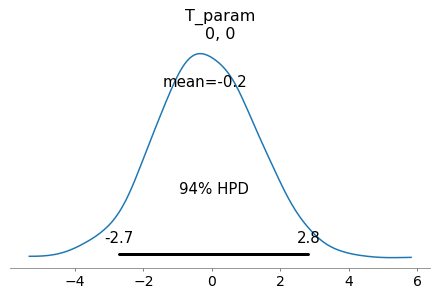
az.plot_posterior(azfit, var_names=['T_param'], coords={'T_param_dim_0':[0], 'T_param_dim_1':[0]});
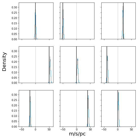
[38]:
fig, ax = plt.subplots(3, 3, figsize=(8, 8), sharex=True, sharey=True)
fig.subplots_adjust(bottom=0.1, top=0.95, right=0.95, left=0.15)
ax = ax.ravel()
for cax, cT, truth in zip(ax, stanfit["T_param"].reshape((-1, 9)).T, cl.T.ravel()):
    cax.hist(cT, bins=32, density=True, histtype="step")
    cax.axvline(truth, c="k")
    cax.axvline(0, c="gray", lw=0.5)
fig.text(0.55, 0.05, "m/s/pc", ha="center", va="center", size=20)
fig.text(0.05, 0.55, "Density", ha="center", va="center", rotation=90, size=20)
fig.savefig("mock_posterior_T.png")
[40]:
az.summary(azfit, var_names=['v0', 'sigv', 'T_param'])
[40]:
| mean | sd | mcse_mean | mcse_sd | hpd_3% | hpd_97% | ess_mean | ess_sd | ess_bulk | ess_tail | r_hat | |
|---|---|---|---|---|---|---|---|---|---|---|---|
| v0[0] | -6.312 | 0.009 | 0.000 | 0.000 | -6.329 | -6.295 | 4194.0 | 4193.0 | 4182.0 | 3104.0 | 1.0 |
| v0[1] | 45.233 | 0.011 | 0.000 | 0.000 | 45.213 | 45.255 | 3715.0 | 3715.0 | 3726.0 | 2801.0 | 1.0 |
| v0[2] | 5.309 | 0.009 | 0.000 | 0.000 | 5.292 | 5.325 | 3736.0 | 3736.0 | 3744.0 | 2761.0 | 1.0 |
| sigv | 0.102 | 0.004 | 0.000 | 0.000 | 0.094 | 0.110 | 4079.0 | 4065.0 | 4091.0 | 2782.0 | 1.0 |
| T_param[0,0] | -0.193 | 1.470 | 0.023 | 0.026 | -2.713 | 2.825 | 4264.0 | 1603.0 | 4248.0 | 2994.0 | 1.0 |
| T_param[0,1] | -49.671 | 1.497 | 0.024 | 0.017 | -52.673 | -47.076 | 4041.0 | 4041.0 | 4047.0 | 2859.0 | 1.0 |
| T_param[0,2] | 18.266 | 1.330 | 0.021 | 0.015 | 15.793 | 20.782 | 4000.0 | 4000.0 | 4002.0 | 2856.0 | 1.0 |
| T_param[1,0] | 53.288 | 1.709 | 0.027 | 0.019 | 49.914 | 56.317 | 4033.0 | 4033.0 | 4037.0 | 2718.0 | 1.0 |
| T_param[1,1] | 3.204 | 1.761 | 0.028 | 0.021 | 0.158 | 6.763 | 3929.0 | 3461.0 | 3938.0 | 2981.0 | 1.0 |
| T_param[1,2] | -38.332 | 1.551 | 0.024 | 0.017 | -41.152 | -35.436 | 4335.0 | 4335.0 | 4326.0 | 3082.0 | 1.0 |
| T_param[2,0] | -19.730 | 1.366 | 0.021 | 0.015 | -22.275 | -17.212 | 4171.0 | 4171.0 | 4169.0 | 2701.0 | 1.0 |
| T_param[2,1] | 42.125 | 1.415 | 0.022 | 0.016 | 39.570 | 44.876 | 4161.0 | 4161.0 | 4166.0 | 3082.0 | 1.0 |
| T_param[2,2] | 2.086 | 1.235 | 0.019 | 0.015 | -0.092 | 4.417 | 4306.0 | 3546.0 | 4309.0 | 2835.0 | 1.0 |
[ ]: